Introduction
Business never stands still, and neither does business data. Every data set is just a snapshot of a business. Each feature in data has a time frame before a snapshot date. Even within a time frame, some data still has temporal dynamics. We'll detail this point using three examples. The first is about historical prices of stock market; the third introduces a paper which shows a subtle temporal nature in beer reviews. The two are described briefly. The second is about the effect of cutoff dates on the target feature in survival analysis.
Adjusted closing prices of stocks
Historical data can change. For example, if we download Apple stock historical data at different time, we might get different adjusted closing prices even during the same time periods because of prices adjustment for dividends and splits.
The effect of cutoff dates on right-cencoring in Kaplan-Meier estimation
Survival analysis estimates how long until a particular event happens. In business a typcial use case is service subscribers' tenure analysis. Here are a few key concepts of survival analysis.
Tenure is censored data, which means the information about tenure is partially known.
Hazard probabilities measure the probability that an event succumbs to a risk at a given time t. The hazard probability at tenure t is the ratio between two numbers:
- Population that succumbed to the risk \(d_j\): The number of customers who stopped at exactly tenure \(t_j\).
- Population at risk \(n_j\): The number of customers whose tenure is greater than or equal to \(t_j\).
Survival is the probability that an event has not succumbed to the risk up to a given time t. In other words, survival accumulates information about the inverse of hazards. The survival at tenure t is the product of one minus the hazards for all tenures less than t.
Kaplan–Meier estimation(aka, KM method, or product-limit estimator) is one of survivial analysis methods. In 1958 Kaplan and Meier showed that it was, in fact, the nonparametric maximum likelihood estimator. This gave the method a solid theoretical justification. The KM estimation defines survival as
Let's look at an example. idata is a sample data of service subscribers.
import pandas as pd
from io import StringIO

# Snippets of subscribers data.
# Null stop_date means the user is right-censored
# censored : 1 - censored; 0 - uncensored
idata = StringIO(
"""
user_id     market      channel      start_date    stop_date    censored
2488577    Market-B    Channel-C3    2008-06-28                    1
2584066    Market-A    Channel-C3    2008-06-28                    1
2574285    Market-A    Channel-C1    2008-11-28                    1
2201921    Market-B    Channel-C3    2008-09-18                    1
2776956    Market-A    Channel-C2    2008-09-28                    1
1891311    Market-B    Channel-C3    2008-09-28                    1
1995282    Market-B    Channel-C1    2008-05-28    2008-10-28      0
2171689    Market-A    Channel-C1    2008-09-02    2008-11-02      0
1597753    Market-A    Channel-C1    2008-10-01    2008-12-21      0
1987770    Market-B    Channel-C2    2008-10-08    2008-12-28      0
""")

df = pd.read_csv(idata, sep='\t', parse_dates=['start_date', 'stop_date'])
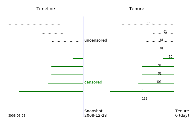
This is right-censored data, which means for currently active users we know when they started, but not when they will stop. Suppose the snapshot date of the data is 2008-12-28. The tenures can be calculated by three variables: start_date, stop_date, and censored.
All the features in the data come from a time frame before a cutoff date. If the cutoff equals to the snapshot date, we can use the data to profile customers during the time frame. Let's use code plotting to illustrate the data.
def plot_right_censor(X, snapshot_date, cutoff_date=None,
                     censored='censored',
                     start='start_date',
                     stop='stop_date'):
    """Plot to illustrate the effect of cutoff on right-censoring.

    Parameters
    ----------

    snapshot_date : str, format: 'yyyy-mm-dd'
        The date when a snapshot of the data was taken.

    cutoff_date : str, default None, format: 'yyyy-mm-dd'
        Define the end of the time frame.
        The default cutoff_date equals to snapshot_date.
        cutoff_date should be earlier than snapshot_date.

    censored, start, stop : str
        The names of columns in DataFrame for censored,
        start_date, and stop_date.
    """
    # code @ https://github.com/geweiwang
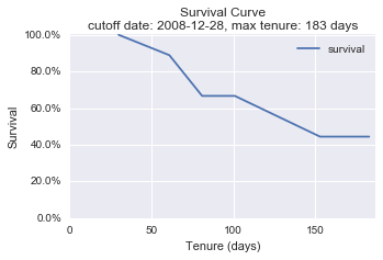
Here is an illustration of the data and its survival curve. We see the default cutoff date equals to the snapshot date.
snapshot_date = '2008-12-28'
plot_right_censor(df, snapshot_date)
|
--- | ---
 |
| 
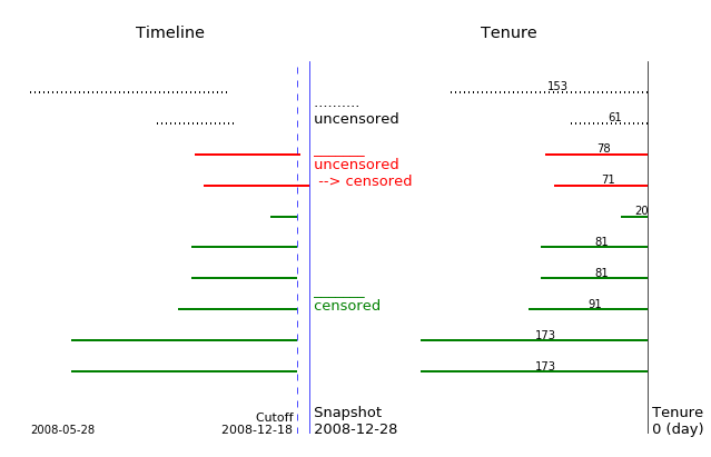
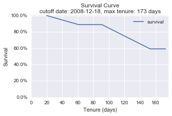
If we set the cutoff date at 2008-12-18, the data and its survival curve change. Two previous uncensored customers become censored.
cutoff_date = '2008-12-18'
plot_right_censor(df, snapshot_date, cutoff_date)
|
--- | ---
 |
| 
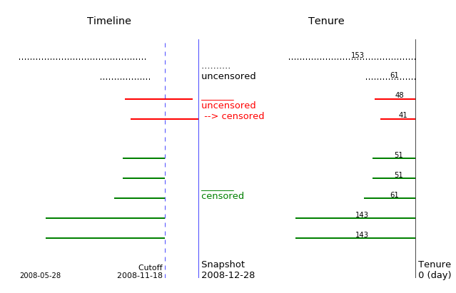
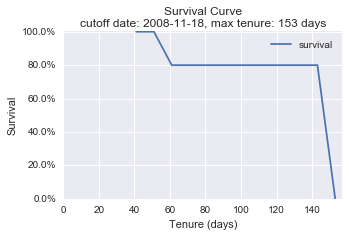
If we move the cutoff date further to 2008-11-18, the data and its survival curve change again. The data of a customer who started the service after the cutoff has been excluded from the KM estimation.
cutoff_date = '2008-11-18'
plot_right_censor(df, snapshot_date, cutoff_date)
|
--- | ---
 |
| 
The changes of numbers of customers are summerized in a table.
Cutoff      | Censored | Uncensored |  Total
------------+----------+------------+--------
2008-12-28  |    6     |     4      |   10
2008-12-18  |    8     |     2      |   10
2008-11-18  |    7     |     2      |    9
We can see the changes of the censored data over the different cutoff dates:
- Some customers come to active again.
- Some customers are excluded from the KM estimation.
- The original profiling data might be used for prediction modeling because the target information comes from a time frame after the new earlier cutoff date.
Next we'll see another example about customers behavior changing with time, but in a little more subtle way.
Customers' beer reviews change with their experience
Customer reviews are traditionally used for sentiment analysis that treats each customer's review history as a series of unordered event. However, when we have big enough data like Amazon customer reviews or RateBeer beer reviews, we have many customers who review multiple times. These customers' tastes may change over time, so do their reviews.
The paper Modeling the Evolution of User Expertise through Online Reviews by Julian McAuley and Jure Leskovec from Stanford digs deep into this kind of data and gets interesting insights on recommending products to customers. They encode temporal information into models via the proxy of user experience.
They demonstrate the evolution of user tastes by analyzing millions of beer reviews. And they find over time some customers grow from 'beer novices' to 'beer experts' and acquire a common taste: hops. Beginners give higher ratings to almost all lagers (less hoppy), while experts give higher ratings to almost all strong ales (more hoppy); thus they conclude that strong ales might be an ‘acquired taste’.
Let's sneak a peak at Amazon customers's beer reviews
- Subset beer-related reviews
- Remove duplicate records
- Filter the data by the number of reviews greater than five
- Stop the default word 'beer', and put the results to an image using word_cloud
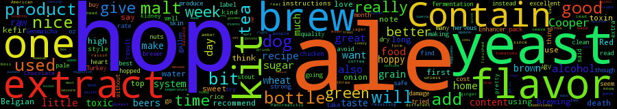
We can see customers with multiple beer reviews talk a lot about 'ale' and 'hop' -- a possible sign of customers having acquired this 'expert' taste over time.
Summary
Through the three examples, we see even during a time frame the data is not static but dynamic.
- Situation changes, so is historical data adjusted to stay aligned with current situation. Adjusted closing prices of stocks are the case.
- For Kaplan-Meier estimation, the censored data changes with cutoff dates moving backward.
- Along customer review timeline there might be latent signals of changing tastes. Recommender systems can extract this temporal feature and model customer evolution for better performance.
Data is almost always dynamic -- some obvious, some subtle. Making good use of the temporal nature of data might give us interesting insights.
Thanks for reading!