Introduction
Test-driven development (TDD) uses agile and lean approaches and test-first practice instead of testing near the end of a development cycle. In this post we will use a simplified example of association rules in retail industry to illustrate TDD in data analysis.
The common metrics for association rules are support, confidence and lift, however, we'll see sometimes these are not enough to ensure rules extracted are correct. Before diving into details, let's give our test-driven data analysis a brief definition:
- Short analysis cycle. Begining with simple cases, we'll generate one-way association rules.
- Use so simple but real data that we can extract rules quickly and check them easily.
- Write a failing test to check the rules.
- Refactor the original code to make the failing test pass.
- [Next iteration]
Generate one-way rules on clean data
Association rules is unsupervised learning techniques which try to find useful patterns in transaction data. The simplest rules are one-way rules, for example, customers buy product A are likely to buy product B at the same time.
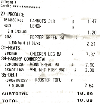
Suppose we have a receipt from a grocery store called Neat, and we'll derive one-way associaton rules for the store using SQL. Let's take a look at the data. The entity-relationship (ER) diagram of Neat data is also given.
| A receipt of store Neat |
The entity-relationship diagram of Neat data |
|---|---|
 |
 |
Insert the Neat data on the receipt into database
SELECT * FROM products_neat; SELECT * FROM orders_neat; SELECT * FROM order_items_neat;
product_id | name             | category       order_id | order_date           order_item_id | order_id | product_id | quantity
-----------+------------------+----------      ---------+-----------           --------------+----------+------------+---------
6148301460 | CARROTS 3LB      | PRODUCE        100      | 2016-01-01             1           | 100      | 6148301460 |  1
4053       | LEMON            | PRODUCE                                          2           | 100      | 4053       |  2
4065       | PEPPER GREEN SWT | PRODUCE                                          3           | 100      | 4065       |  1
2193860    | CHICKEN LEG BA   | MEATS                                            4           | 100      | 2193860    |  1
6340002536 | WOND BREAD WW    | BAKERY                                           5           | 100      | 6340002536 |  1
6340011169 | WHL WHT FIBR BRD | BAKERY                                           6           | 100      | 6340011169 |  1
5719732951 | ROOSTER TOFU     | DELI                                             7           | 100      | 5719732951 |  3
One-way association rules for Neat
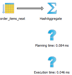
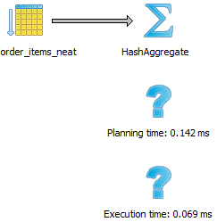
Because of the data schemas of Neat, the three SQL commands give us the same results but use different execution time.
only SELECT |
using GROUP BY |
using DISTINCT |
|---|---|---|
SELECT order_id, product_id FROM order_items_neat; |
SELECT order_id, product_id FROM order_items_neat GROUP BY order_id, product_id; |
SELECT DISTINCT order_id, product_id FROM order_items_neat; |
 |
 |
 |
The three commands give the same result
order_id | product_id
---------+-----------
 100     | 6148301460
 100     | 4053
 100     | 4065
 100     | 2193860
 100     | 6340002536
 100     | 6340011169
 100     | 5719732951
We see the SQL with only SELECT is faster than the one using GROUP BY, which is faster than the one using DISTINCE. The data used here is just one transaction. When we have millions of tranaction records, the difference could be even more pronounced. So we decide to use the SQL without GROUP BY or DISTINCT in the common table expression (CTE) baskets.
/*
Extract one-way association rules for stores Neat and Messy.
Compare the differences between no GROUP BY and using GROUP BY in CTE baskets
Only change the CTE baskets for different scenarios.
The CTE rules and the main SELECT clause are common parts.
*/

WITH baskets AS (
    -- baskets of store Neat
    -- without GROUP BY or DISTINCT
    SELECT oi.order_id, oi.product_id, p.name,
           count(*) OVER (PARTITION BY oi.product_id) AS cnt,
           tot_order
    FROM order_items_neat oi
        INNER JOIN products_neat p ON oi.product_id = p.product_id
        CROSS JOIN (SELECT COUNT(DISTINCT order_id) tot_order FROM order_items_neat) t
),

-- The code below is common for different baskets
rules AS (
    -- ls: left sides of association rules
    -- rs: right sides of association rules
    SELECT ls.product_id AS ls_pid, rs.product_id AS rs_pid,
           ls.name AS ls_name, rs.name AS rs_name,
           count(*) AS cnt_ls_rs,
           max(ls.cnt) AS cnt_ls, max(rs.cnt) AS cnt_rs,
           max(ls.tot_order) AS tot_order
    FROM baskets ls JOIN
         baskets rs ON ls.order_id = rs.order_id
                   AND ls.product_id != rs.product_id
    GROUP BY ls.product_id, rs.product_id, ls_name, rs_name
)
SELECT format('%-20s => %20s', ls_name, rs_name) AS rules,
       round(1.0 * cnt_rs / tot_order, 2) AS expectation,   -- Expectation of right side
       round(1.0 * cnt_ls_rs / tot_order, 2) AS support,    -- Support of the rule: {left side} => {right side}
       round(1.0 * cnt_ls_rs / cnt_ls, 2) AS confidence,    -- Confidence of the rule
       round(1.0 * cnt_ls_rs * tot_order / (cnt_ls * cnt_rs), 2) AS lift  -- Lift of the rule
FROM rules
ORDER BY lift DESC, confidence DESC, support DESC;
As we expect, all values of three metrics (support, confidence, and lift) are 1 because we only have one order. The first three rows are:
                   rules                     | expectation | support | confidence | lift
---------------------------------------------+-------------+---------+------------+------
CARROTS 3LB          =>   PEPPER GREEN SWT   | 1.00        | 1.00    | 1.00       | 1.00
LEMON                =>   CARROTS 3LB        | 1.00        | 1.00    | 1.00       | 1.00
ROOSTER TOFU         =>   PEPPER GREEN SWT   | 1.00        | 1.00    | 1.00       | 1.00
Write a failing test
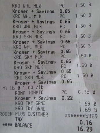
Suppose Neat has acquired another grocery store called Messy. We'll apply the code of Neat to the data of Messy to see if it works. Let's look at the new data.
| A receipt of store Messy |
The entity-relationship diagram of Messy data |
|---|---|
 |
 |
We can see two receipts represent different database schemas.
Insert the Messy data on the receipt into database
SELECT * FROM products_messy; SELECT * FROM orders_messy; SELECT * FROM order_items_messy;
product_id | name         | category          order_id | order_date             order_item_id | order_id | product_id | quantity
-----------+--------------+----------         ---------+-----------             --------------+----------+------------+---------
2305       | KRO WHL MLK  | DAIRY             200      | 2016-01-01               1           | 200      | 2305       |  1
2306       | KRO SKM MLK  | DAIRY                                                 2           | 200      | 2305       |  1
2307       | ROMA TOMATO  | PRODUCE                                               3           | 200      | 2305       |  1
2308       | KRO TKY GRND | NA                                                    4           | 200      | 2305       |  1
                                                                                  5           | 200      | 2306       |  1
                                                                                  6           | 200      | 2306       |  1
                                                                                  7           | 200      | 2306       |  1
                                                                                  8           | 200      | 2306       |  1
                                                                                  9           | 200      | 2307       |  1
                                                                                 10           | 200      | 2308       |  1
                                                                                 11           | 200      | 2308       |  1
Then we apply the SQL code of Neat to the Messy data. We only need to change the common table expression (CTE) baskets to:
WITH baskets AS (
    -- baskets of store Messy
    -- without GROUP BY or DISTINCT
    SELECT oi.order_id, oi.product_id, p.name,
           count(*) OVER (PARTITION BY oi.product_id) AS cnt,
           tot_order
    FROM order_items_messy oi
        INNER JOIN products_messy p ON oi.product_id = p.product_id
        CROSS JOIN (SELECT COUNT(DISTINCT order_id) tot_order FROM order_items_messy) t
),
However, we get obvious wrong results (the first three rows shown here):
                    rules                      | expectation | support | confidence | lift
-----------------------------------------------+-------------+---------+------------+------
KRO SKM MLK          =>   KRO WHL MLK          | 4.00        | 16.00   | 4.00       | 1.00
KRO WHL MLK          =>   KRO SKM MLK          | 4.00        | 16.00   | 4.00       | 1.00
KRO TKY GRND         =>   KRO WHL MLK          | 4.00        | 8.00    | 4.00       | 1.00
All values are supposed to be 1 with only one order. The good news is that we now have a failing test case. Let's figure out what's wrong with the original code.
The CTE baskets is the building block for generating the rules. Its data pipeline is:

The wrong counting happens in the window function, which is in the last step. We want the windown function to calculate the total number of each unique product_id in each order.
If we use PostgreSQL and try count(DISTINCT oi.product_id) OVER (PARTITION BY oi.product_id) AS cnt, we get ERROR: DISTINCT is not implemented for window functions. So the product_id has to be unique for each order_id before being piped into the window function. A common practice is to use GROUP BY.
Refactor the original code
Change the common table expression baskets to:
WITH baskets AS (
    -- baskets of store Messy
    -- using GROUP BY
    SELECT oi.order_id, oi.product_id, p.name,
           count(*) OVER (PARTITION BY oi.product_id) AS cnt,
           max(tot_order) AS tot_order
    FROM order_items_messy oi
        INNER JOIN products_messy p ON oi.product_id = p.product_id
        CROSS JOIN (SELECT COUNT(DISTINCT order_id) tot_order FROM order_items_messy) t
        GROUP BY oi.order_id, oi.product_id, p.name
),
After refactoring we get correct output (the first three rows shown here):
                    rules                      | expectation | support | confidence | lift
-----------------------------------------------+-------------+---------+------------+------
KRO TKY GRND         =>   KRO WHL MLK          | 1.00        | 1.00    | 1.00       | 1.00
KRO SKM MLK          =>   KRO TKY GRND         | 1.00        | 1.00    | 1.00       | 1.00
KRO TKY GRND         =>   KRO SKM MLK          | 1.00        | 1.00    | 1.00       | 1.00
Now we have passed the failing test!
During the first iteration, we have known the data, built a basic association rules extracting function, written a failing test, and refactored the code to pass it. All of these actions are quick and lean. We are now comfortable to move on with more data or extracting complex rules. And remember: writing failing tests for each iteration.
Summary
We have used an example to illustrate how data analysis can work hand in hand with testing to explore and produce results early and often. TDD even advocates writing tests first before coding. Though we don't always have time budget and resources to do this kind of TDD, and during the exploratory phase testing might not be necessary, we keep TDD in mind and practice it if necessary for at least three reasons:
- Writing test cases is a process of clarifying objectives of data analysis, and documenting how the code is intended to work. As code becomes more complex, the need for documentation increases.
- TDD can help mitigate the fear and error of refactoring, modifying features, or adding new features. With test cases, we don't do them at the mercy of luck.
- When switching from exploratory data analysis phase to production phase, the agile way of TDD can ensure that our data products are on the right track.
Thanks for reading!